# Pr(theta>2)
1-pexp(2,3)
[1] 0.002478752# Monte Carlo simulations
set.seed(2024)
N <- 1000000
samples <- rexp(N,3)
P <- mean(samples > 2)
print(P)[1] 0.002496chapter 3
Let prior uncertainty about a parameter \(\theta\) be reflected by the density
\[ p(\theta) = ce^{−3\theta} I(0,\infty)(\theta). \]
Find the constant c that makes this integrate to one. Also find \(Pr(\theta > 2)\) and \(Pr(\theta > 4 | \theta > 2)\). Find the median and the expected value. Finally, obtain a 95% probability interval for \(\theta\)
let \(\frac{c}{3}=1\),then we have \(c=3\)
let \(x=2\), then we have
\[ Pr(\theta>2) = e^{-3*2} = 0.002478752 \]
\[ Pr(\theta > 4 | \theta > 2) = \frac{Pr(\theta > 4)*Pr(\theta > 2 | \theta > 4)}{(\theta > 2)} = \frac{Pr(\theta > 4)}{(\theta > 2)} = e^{-3*2} = 0.002478752 \]
# Pr(theta>2)
1-pexp(2,3)[1] 0.002478752# Monte Carlo simulations
set.seed(2024)
N <- 1000000
samples <- rexp(N,3)
P <- mean(samples > 2)
print(P)[1] 0.002496# Pr(theta>4|theta>2)
(1-pexp(4,3))/(1-pexp(2,3))[1] 0.002478752For Exp(3) , \(Mean = \frac{1}{\theta}\) ,\(Mdian = \frac{Ln2}{\theta}\), We all know \(\theta =3\), so we have \(Mean = \frac{1}{3}\) , \(Median = \frac{Ln2}{3}\)
95% probability interval for \(\theta\)
qexp(c(0.025,0.975),3)[1] 0.008439269 1.229626485Suppose \(n\) cities were sampled and for each city \(i\) the number \(y_i\) of deaths from ALS were recorded for a period of one year. We expect the numbers to be Poisson distributed, but the size of the city is a factor. Let \(M_i\) be the known population for city \(i\) and let
\[ y_i|\theta ~ Pois(\theta M_i), i= 1,...k \]
where \(\theta\) > 0 is an unknown parameter measuring the common death rate for all cities. Given \(\theta\), the expected number of ALS deaths for city i is \(\theta M_i\), so \(\theta\) is expected to be small. Assume that independent scientific information can be obtained about \(\theta\) in the form of a gamma distribution, say \(Gamma(a, b)\). Show that this prior and posterior are conjugate in the sense that both have gamma distributions.
\[ \theta ~ Gamma(a,b) \Rightarrow p(\theta) = [b^a/\Gamma(a)]\theta^{a-1}e^{-b\theta}I_{(0,\infty)}(\theta) \]
\[ y_i|\theta~Pois(\theta M_i)\Rightarrow P(y_i|\theta) = \frac{(\theta M_i)^{Y_i}e^{-\theta M_i}}{Y_i!} \]
\[ L(\theta)= (\prod \frac{M_{i}^{y_i}}{y_i !}) \theta^{\sum y_i} e^{-\theta \sum M_i } \]
\[\begin{align} p(\theta|y) & \propto p(\theta)L(\theta) \\ & \propto \theta^{a-1}e^{-b\theta}\theta^{\sum y_i} e^{- \theta \sum M_i} \\ & \propto \theta^{a+\sum y_i -1} e^{- \theta (b+\sum M_i)} \end{align}\]Finally, we have
\[ \theta|y ~ Gamma(a+\sum y_i ,b+\sum M_i) \]
Extending Exercise 3.2, two cities are allowed different death rates. Let \(y_i ~ Pois(θ_i M_i), i = 1, 2,\) where the \(M_is\) are known constants. Let knowledge about \(θ_i\) be reflected by independent gamma distributions, namely \(θ_i ∼ Gamma(a_i, b_i)\). Derive the joint posterior for \((\theta_1,\theta_2)\). Characterize the joint distribution as we did for sampling two independent binomials. Think of \(\theta_i\) as the rate of events per 100 thousand people in city \(i\). For independent priors \(\theta_i ∼ Gamma(1, 0.1)\), give the exact joint posterior with \(y_1 = 500, y_2 = 800\)in cities with populations of 100 thousand and 200 thousand, respectively.
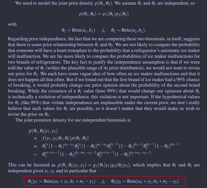
\[ P(\theta_1 , \theta_2)=p_1(\theta_1)p_2(\theta_2) \]
According to the above conclusion, we have
\[ \theta_1,\theta_2 ~ Gamma(a + y_1,b+M_1)Gamma(a + y_2,b+M_2) \]
We know,
\[\begin{align} a_1 = a_2 &= 1 \\ b_1 = b_2 &= 0.1 \\ y_1 &= 500 \\ y_2 &= 800 \\ M_1 &= 100 \\ M_2 &= 200 \end{align}\]Finally,
\[\begin{align} p(\theta_1,\theta_2|y_1 =500,y_2=800)=[[100.1^{501} / \Gamma(501)]\theta_1 ^{500}e^{-100.1\theta_1}][[200.1^{801} / \Gamma(801)]\theta_2 ^{800-1}e^{-200.1\theta_2}] \end{align}\]


Perform Example 3.1.3 in WinBUGS with \(y_1 ∼ Bin(80,\theta1)\), \(y_2 ∼ Bin(100,\theta_2)\) \(\theta1 ∼ Beta(1, 1), \theta 2 ∼ Beta(2, 1)\) with observations \(y_1 = 32\) and \(y_2 = 35\). Put each term in the model on a separate line. There should still be only two list statements with entries separated by commas. See Exercises 3.6 and 3.7 for WinBUGS syntax.
suppressMessages(library(rjags))

# step(x) : test for x > = 0 logical

model_string <- "
model {
  # Likelihood
  y1 ~ dbin(theta1, n1)
  y2 ~ dbin(theta2, n2)

  # Priors
  theta1 ~ dbeta(1, 1)
  theta2 ~ dbeta(2, 1)

  # Derived parameter
  gamma <- theta1 - theta2
  p <- step(theta1 - theta2)
}
"

data_list <- list(
    y1 = 32,
    n1 = 80,
    y2 = 35,
    n2 = 100
)


jags_model <- jags.model(
    textConnection(model_string),
    data = data_list,
    n.chains = 1,
    n.adapt = 1000
)
Compiling model graph
Resolving undeclared variables
Allocating nodes
Graph information:
Observed stochastic nodes: 2
Unobserved stochastic nodes: 2
Total graph size: 10
Initializing modelupdate(jags_model, 1000)
mcmc_samples <- coda.samples(
model = jags_model,
variable.names = c("theta1", "theta2", "gamma",'p'),
n.iter = 10000
)
head(mcmc_samples[[1]])Markov Chain Monte Carlo (MCMC) output:
Start = 2001
End = 2007
Thinning interval = 1
gamma p theta1 theta2
[1,] 0.023010830 1 0.4000277 0.3770169
[2,] 0.018173025 1 0.3901233 0.3719502
[3,] 0.003834567 1 0.3489312 0.3450966
[4,] 0.018618141 1 0.4363264 0.4177083
[5,] 0.101206763 1 0.4050952 0.3038884
[6,] 0.039708602 1 0.3476874 0.3079788
[7,] 0.112117808 1 0.4311559 0.3190381mean(mcmc_samples[[1]][,'p'])[1] 0.7259# 还可以拿出来直接算
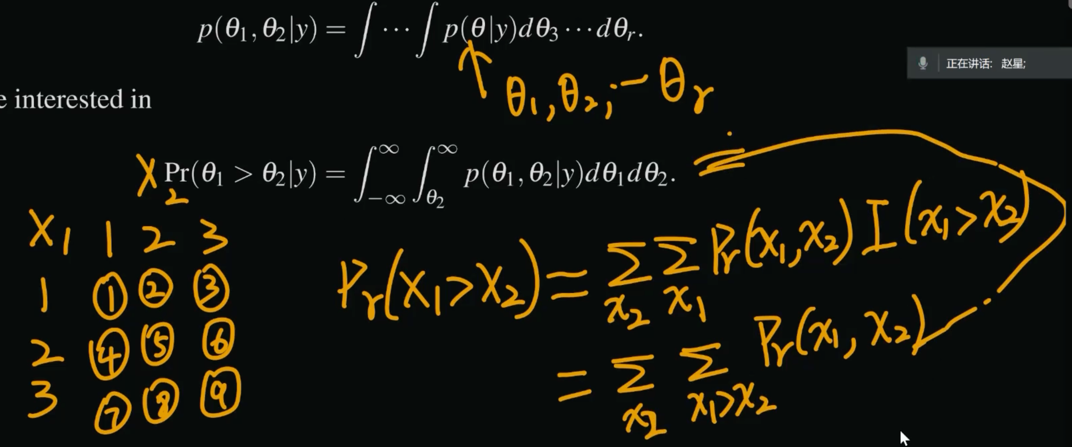
mean(mcmc_samples[[1]][,'theta1']>=mcmc_samples[[1]][,'theta2'])[1] 0.7259# 知道后验分布 直接蒙特卡洛算
data <- list(n1=80,n2=100,
a1=1,b1=1,
a2=2,b2=1,
y1=32,y2=35)
nsim <- 1000
rtheta1 <- rbeta(nsim,
data$a1 + data$y1,
data$b1 + data$n1 - data$y1,
)
rtheta2 <- rbeta(nsim,
data$a2 + data$y2,
data$b2 + data$n2 - data$y2,
)
mean(rtheta1>=rtheta2)[1] 0.732Perform a data analysis for the model in Exercise 3.3 using the data \(y_1 = 500\), \(y_2 = 800\), \(M_1 = 100\), \(M_2 = 200\), and using independent \(Gamma(1, 0.01)\) priors for the \(θ_is\). Make WinBUGS based inferences for all parameters and functions of parameters discussed there using a Monte Carlo sample size of 10,000 and a burn-in of 1,000. This may involve an excursion into the “Help” menu to find the syntax for Poisson and gamma distributions. Compare the posterior means for \(\theta_1\) and \(\theta_2\) based on the WinBUGS output to the exact values from the Gamma posteriors that you obtained in Exercise 3.3.
model_string <- "
model {
    y1 ~ dpois(theta1*M1)
    y2 ~ dpois(theta2*M2)

    theta1 ~ dgamma(a, b)
    theta2 ~ dgamma(a, b)
}
"

data_list <- list(
    a = 1,
    b = 0.01,
    y1 = 500,
    M1 = 100,
    y2 = 800,
    M2 = 200
)

jags_model <- jags.model(
    textConnection(model_string),
    data = data_list,
    n.chains = 1,
    n.adapt = 10000
)
Compiling model graph
Resolving undeclared variables
Allocating nodes
Graph information:
Observed stochastic nodes: 2
Unobserved stochastic nodes: 2
Total graph size: 10
Initializing modelupdate(jags_model, 1000)
mcmc_samples <- coda.samples(
model = jags_model,
variable.names = c("theta1", "theta2"),
n.iter = 10000
)
head(mcmc_samples[[1]])Markov Chain Monte Carlo (MCMC) output:
Start = 1001
End = 1007
Thinning interval = 1
theta1 theta2
[1,] 4.855552 4.025151
[2,] 4.852221 4.008059
[3,] 5.160709 3.929361
[4,] 4.924075 4.312788
[5,] 4.952397 3.982148
[6,] 4.760714 3.999971
[7,] 5.021981 4.076147apply(mcmc_samples[[1]],2,mean) theta1 theta2
5.010653 4.006890 # gamma分布均值为a/b 套用3.3中后验分布的结果
501/100.1[1] 5.004995801/200.1[1] 4.002999
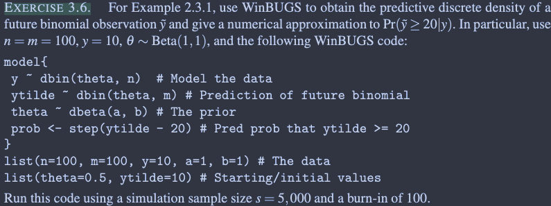
model_string <- "
model {
    y ~ dbin(theta , n)
    ytilde ~ dbin(theta, m)
    theta ~ dbeta(a, b)
    prob <- step(ytilde - 20)
}
"

data_list <- list(n=100, m=100, y=10, a=1, b=1)

jags_model <- jags.model(
    textConnection(model_string),
    data = data_list,
    n.chains = 1,
    n.adapt = 1000
)
Compiling model graph
Resolving undeclared variables
Allocating nodes
Graph information:
Observed stochastic nodes: 1
Unobserved stochastic nodes: 2
Total graph size: 10
Initializing modelupdate(jags_model, 1000)
mcmc_samples <- coda.samples(
model = jags_model,
variable.names = c("theta",'prob','ytilde'),
n.iter = 10000
)
apply(mcmc_samples[[1]],2,mean) prob theta ytilde
0.0377000 0.1079444 10.7894000 # 不在JAGS里面算预测分布及概率的话可以这样
nsim <- 10000
# 预测分布
ytilde <- rbinom(nsim,
size = 100,# 每次试验重复100次对应前面的m=100
prob = mcmc_samples[[1]][,'theta']
)
mean(ytilde)[1] 10.7913# y>=20概率
mean(ytilde>=20)[1] 0.0359mean(mcmc_samples[[1]][,'ytilde']>=20)[1] 0.0377
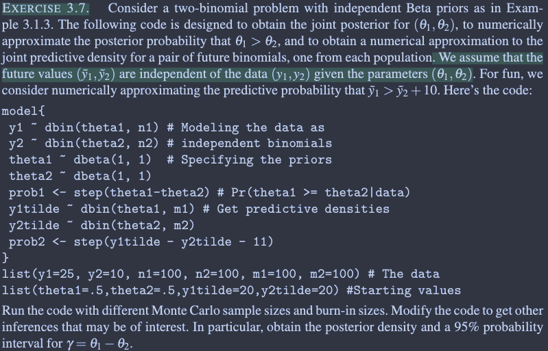
model_string <- "
model{
  y1 ~ dbin(theta1, n1)
  y2 ~ dbin(theta2, n2)
  theta1 ~ dbeta(1, 1)
  theta2 ~ dbeta(1, 1)
  prob1 <- step(theta1-theta2)
  y1tilde ~ dbin(theta1, m1)
  y2tilde ~ dbin(theta2, m2)
  prob2 <- step(y1tilde - y2tilde - 11)
  gamma <- theta1-theta2
}
"
data_list <- list(y1=25, y2=10, n1=100, n2=100, m1=100, m2=100)

jags_model <- jags.model(
    textConnection(model_string),
    data = data_list,
    n.chains = 1,
    n.adapt = 1000
)
Compiling model graph
Resolving undeclared variables
Allocating nodes
Graph information:
Observed stochastic nodes: 2
Unobserved stochastic nodes: 4
Total graph size: 17
Initializing modelupdate(jags_model, 1000)
mcmc_samples <- coda.samples(
model = jags_model,
variable.names = c("theta1","theta2",'prob1','prob2','gamma','y1tilde','y2tilde'),
n.iter = 1000
)
apply(mcmc_samples[[1]],2,mean) gamma prob1 prob2 theta1 theta2 y1tilde y2tilde
0.1490780 0.9950000 0.7370000 0.2561037 0.1070257 25.8040000 10.6490000 quantile(mcmc_samples[[1]][,'gamma'],c(0.025,0.975)) 2.5% 97.5%
0.03813197 0.25362877